Strategic Assessment: Supply Chain
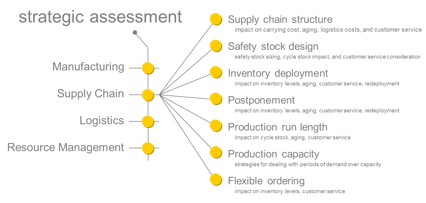
Here are the primary problem areas SDI has assessed:
- Supply chain structure impact on carrying cost, aging, logistics costs, and customer service
- Safety Stock Design safety stock sizing, cycle stock impact, and customer service consideration
- Inventory Deployment impact on inventory levels, aging, customer service, redeployment
- Postponement impact on inventory levels, aging, customer service, redeployment
- Production run length impact on cycle stock, aging, customer service
- Production Capacity strategies for dealing with periods of demand over capacity
- Flexible Ordering impact on inventory levels, customer service
Supply Chain Structure
Summary
The simple question: who gets what from where? leads to a broad set of questions of supply chain structure. These could be grouped as follows:
- How many echelons of supply are there [example: should a manufacturing company have regional warehouses or ship direct to customer distribution centers]
- How segregated or integrated should sourcing be [example: should each plant make every product, or should plants specialize around a few products]
- How flexible should sourcing be [example: should customers be able to order from multiple plants; should product be redeployed from one regional warehouse to another]
Alternative supply chain structures are often generated by optimization packages. Simulation is then able to assess the dynamic performance of proposed alternatives.
Paper: Combined Use of Optimization and Simulation Technologies to Design and Optimal Logistics Network; Glenn Wegryn, Procter & Gamble; Andy Siprelle, Simulation Dynamics. CLM Conference, 2001
Echelons
Addition or subtracting stages of distribution. A stage of distribution can be defined by a cross docking operation or by a warehouse where product inventory is maintained. In both cases, economies of scale are achieved in shipping. When an inventory is maintained, downstream orders are filled with shorter Lead times, reducing the inventories that have to be maintained downstream.
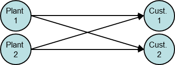
DIRECT SHIPMENT: Simplifies shipping and handling but requires larger inventories at both ends to support larger shipment amounts and longer order lead times.
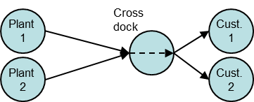
CROSS DOCKING: Consolidates plant loads allowing more frequent and smaller orders and reducing shipping costs.
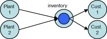
REGIONAL DISTRIBUTION CENTER: Supports rapid customer order filling, more frequent and smaller orders. Additional inventories may increase inventories overall. Increased handling costs.
Product Mix & Sourcing
| Product Mix | Pros | Cons |
|---|---|---|
| Segregated Each product made at only one plant |
Longer production runs; simplified scheduling; fewer changeovers; products made at most efficient plants | Greater shipping distances; potential misallocation problems. No ability to use alternate plants for periods of demand over capacity |
| Integrated Products made regionally at multiple plants |
Shorter shipping distances; ability to shift production to alternate plants when regional demand exceeds production | Shorter production runs; more production changeovers; more complex production scheduling |
Safety Stock Design
Summary
Safety stock protects an inventory against out-of-stocks resulting from variability in demand or supply. Under idealized supply and demand conditions, safety stock levels can be calculated as a function of customer service goals, resupply time and demand variability.
- Increased demand variability: increased safety stock
- Increased order lead time: increased safety stock
- Increased case fill goal: increased safety stock
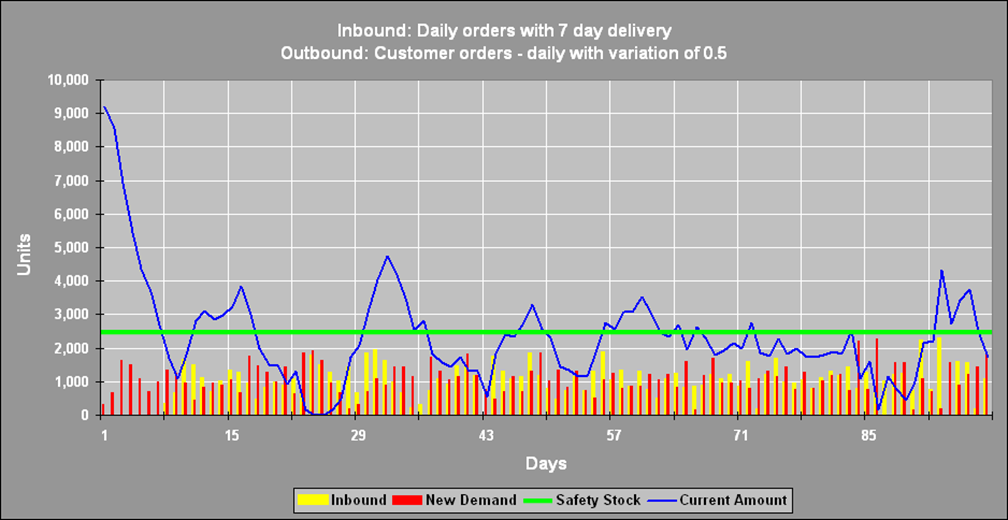
This plot shows safety stock of 2500 units with daily demand forecasted at 1000 units, lead time of 7 days and a case fill goal of 98%. The fact that the inventory level approaches zero several times is an indication that safety stock is properly sized.
Safety Stock Reduction
There are several strategies for reduction of safety stock. Simulation is a powerful tool for assessing the effectiveness of these alternatives.
- Combine fixed and variable safety stock
- Experience at Simulation Dynamics has shown that a 50/50 mix of fixed and variable safety stock is better than 100% fixed or 100% variable
- Flexible ordering capabilities - SDI has conducted extensive research demonstrating up to 77% of maximum potential safety stock savings through strategic flexible ordering contract design. See Supply Chain: Flexible ordering for detailed methodology and proven results.
- Increase in customer service time
- The time between when a customer order is placed and when it is shipped
- Order differentiation
- Offer different customer service time contracts based on product category (for example: A, B C Classes)
- Reduction of order fill lead time
- Expedited orders
- Additional distribution echelon
Baseline Calculation
Under idealized supply and demand conditions, safety stock levels can be calculated as a function of customer service goals, resupply time and demand variability. This calculation provides a baseline which can be modified to take into account complicating factors.
safety stock units = demand x Std Dev x k x √ resupply time
Demand: The periodic (daily, weekly, etc) forecasted demand
Std Dev: normalized standard deviation of forecast compared to demand
k: The value of k is the inverse standard normal cumulative distribution for the desired percent orders filled.
- goal of 95%: k = 1.645 std devs above mean
- goal of 98%: k = 2.054
- goal of 99%: k = 2.326
Resupply time: Number of periods (days, weeks, etc) to fill resupply orders
Safety stock can be expressed in periods (such as '5 days of safety stock') by dropping the demand variable from the equation.
Complicating Factors
Several factors can require that the basic safety stock equation be modified, or entirely replaced with empirical safety stock sizing.
- Impact of Cycle Stock
The basic equation for safety stock assumes that orders will be placed periodically (daily, weekly) to maintain inventory levels at or above the calculated safety stock level. Deliveries to the inventory may be supplemented by cycle stock that results from long production runs at the supplier, or economic order size considerations. This chart illustrates a case where safety stock has been calculated at 66 units. However, the product is ordered in lots of 1000 units. With demand of 100 units per day, orders are placed on a 10 day cycle. Realistically, the inventory could only stock-out on the last day or two of the ordering cycle. Since the 66 unit safety stock is derived from the basic equation, it assumes daily reordering and the possibility of running out on any day. As a result the safety stock is over sized.
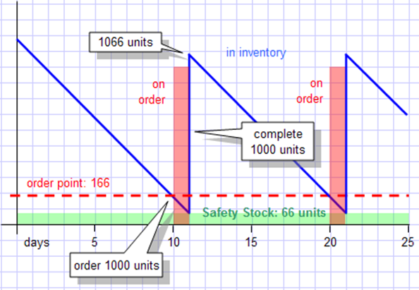
If the original safety stock was based on a order fill goal of 99%, a new safety stock level could be roughly calculated based on a goal of 90%, since there is only one out of 10 days on which a stock out could occur.
Note that in this example the order cycle is not a fixed period. If the inventory gets to its order point in 8 days, an order for 1000 units will be placed.
- Delivery Delays
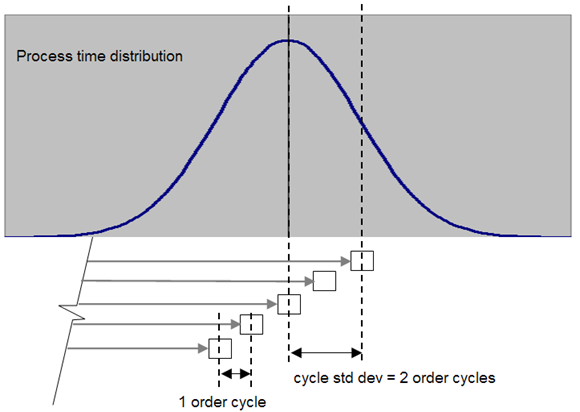
There are many potential causes of variation in delivery times. For this discussion, we assume causes of delay which can be characterized by a standard deviation. The critical factor in this analysis is not how late any individual shipment is, but rather, how many shipments might be late at any one time. For example, if the probability of 6 shipments being late is within the service performance goal of a node, then safety stock must be provided to cover this possibility.
The critical factor in determining the number of shipments that might be late at any one time is the ratio of the delivery time standard deviation to the order cycle. For example if the standard deviation of the deliver time is 4 days, and orders are placed every two days, then the cycle standard deviation is 2 cycles. The average process duration is not relevant to this calculation. The same cycle standard deviation would result from a process duration standard deviation of 14 days and an order cycle of 7 days.
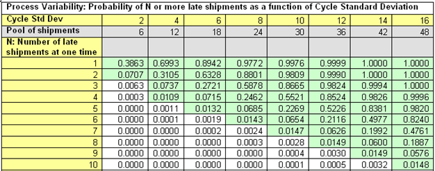
Once the cycle standard deviation is known, the probability of N shipments being late can be approximated, where N can be any combination of shipments. The table below gives this approximation for values of N from 1 to 10 and cycle standard deviations from 2 to 16. The shaded area indicates numbers of late shipments that must be protected by safety stock.
- Fixed reorder cycle
In the case illustrated below, orders are placed every 10 days. Forecasted demand is 100 units per day. The calculated safety stock of 66 units was based on the assumption that orders will be placed every day to cover forecasted demand AND the forecast error of the prior day. As can be seen in the first order cycle below, demand for the period was 1150 units, 150 over forecast. Stock ran out in the middle of the 9th day of the cycle.
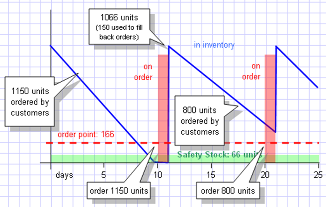
The effect of a fixed order cycle is to add the number of days in the cycle to the reorder time. The amount of stock ordered for each cycle must be sufficient to cover forecast error for the entire time until the next delivery.
- Fill rate goal
Safety stock design algorithms are based on specification of order fill rate where total orders are divided into orders filled on time. 'Orders' here refers to line item orders. Modeled supply chain performance can be weighted by order size or value.
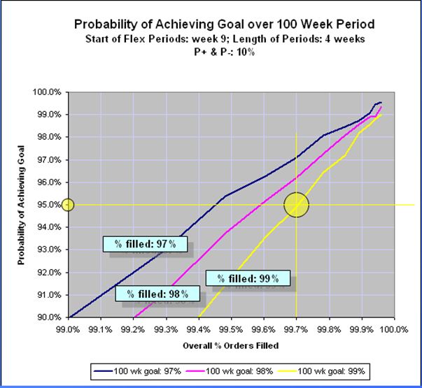
Life cycle order fill performance may require two levels of analysis. In the example show in the graph, a product has a 100 week life. The customer goal is to have a 95% probability that the fill rate for this product will be at or above 99%. The yellow plot shows that to achieve 99% fill rate 95% of the time, an average performance of 99.7% would be required.
- Intermittent demand The challenge presented by intermittent demand is that demand events will occur earlier than average, before stock has arrived to cover it. For this reason substantially increased safety stock is required based on calculations of how many excess demand events will occur during the lead time period. An algorithm has been developed to make this calculation both at customer facing inventories and at nodes which supply customers with varying patterns of demand. The logic is summarized below.
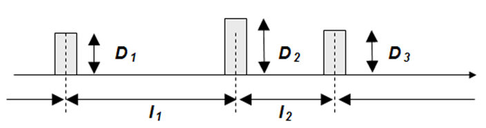
Be ready for the next demand event: At any given time there must be sufficient safety stock on hand to meet the next demand event. This amount can be computed based on the target percent orders filled, the mean demand amount and the normal distribution of the demand event interval.
Cover EXCESS demand events: if a demand event occurs before stock is delivered that was intended to meet it, there will be a missed order unless there is stock on hand to cover that amount. For example, say the mean demand interval is 10 days, and the procurement time for the inventory is 10 days. Nominally, safety stock could be sized to meet a single demand event assuming that the next shipment will be received before the next demand event. But since there is variation in the demand interval, the next demand event might well occur before the 10 day procurement time has elapsed. Therefore, there must be stock to cover two demand events.
Depending on the interval variation, there might be additional demand events during the procurement time. A computation method has been designed to determine the stock required to cover interval variation as a function of lead time, mean interval, and interval variation.
- Capacity constraints Safety stock is an inappropriate solution to the problem of periodic capacity constraints. Alternative approaches for dealing with capacity constraints are discussed in this document at Production Capacity.
To the extent that pre-building of reserves for periods of high demand creates additional stock at zero service time inventories, safety stocks can be reduced for the same reasons as discussed under Impact of cycle Stock for customers.
Case Studies
- Downstream Packaging Model The baseline safety stock calculation, modified to account for fixed weekly downstream packaging schedules, accurately predicted safety stock requirements at customer facing inventories in this model.
- Inventory Deployment Model The baseline safety stock calculation provided a starting point for substantial empirical adjustments of safety stock at customer facing inventories. This was required as a result of long production cycles with cycle stock pushed downstream, instances of significant intermittent demand, and use of redeployment from DC to DC.
- Revolutionary Supply Chain Understanding - General Mills This is a very similar study to that done for the Inventory Deployment model.
- Chemical Packaging Model Safety stock was set at customer facing inventories using the basic calculation, without modification.
Inventory Deployment
Summary
In many industries, economies of scale dictate that production runs far exceed immediate demand. The resulting cycle stock must be deployed at some stage of the supply chain. The pros and cons of deployment options are a function of production cycle length, forecast variability, redeployment costs, and aging factors.
Papers:
- Supply chain simulation software II: benefits of using a supply chain simulation tool to study inventory allocation. Siprelle, Parsons, Clark. Winter Simulation Conference 2003
- Tactical logistics and distribution systems (TLoaDS) simulation. Parsons, Krause, winter Sim 1999
Pros & Cons
| Deployment | Pros | Cons |
|---|---|---|
| Upstream | Risk pooling: variability of downstream demand is pooled when stock is held upstream. Stock held upstream can be used to fill out partial truck loads. | Upstream storage costs may be higher. Higher levels of safety stock may be required downstream. |
| Downstream | Downstream cycle stock will minimize the need for safety stock. Out of stocks can only occur at the end of each production cycle. Downstream storage costs may be lower. | Misallocation: cycle stock pushed downstream must be allocated among downstream locations on the basis of forecasts. Stock may have to be redeployed from one downstream location to another. |
Case Studies
- Inventory Deployment Model The principal strategic question addressed by this model was the impact of upstream vs. downstream deployment of cycle stock on four system performance factors: total inventories, customer service, DC to DC redeployment, and disposal of over aged product.
- Downstream Packaging Model A relatively minor issue in this case study was the question of where to deploy cycle stock of the bulk material shipped downstream for packaging. We concluded that it was most cost effective to keep all cycle stock upstream at the plants and fill orders from distribution centers on a pull order basis.
Postponement
Summary
The goal of postponement is to reduce the supply chain response time to customer orders. This allows substantial reduction of finished product inventories. Typically, many finished products are made from a relatively few basic products. By moving the assembly, packaging or labeling of products downstream, the core inventories downstream can be few basic products, with finished items produced in direct response to local demand.
Postponement can be implemented as a matter of degree along three axes:
- What operations do we push downstream?
- Examples: labeling, packaging, final product assembly, component assembly
- How far downstream do we push them?
- Examples: to national DC's, to regional DC's, to customer DC's
- What products do we push downstream?
- Examples: low volume products, products with volatile demand
Pros & Cons
All forms of postponement have costs and benefits. These often vary by product category. Simulation can provide assessment of the costs and benefits of a wide range of postponement alternatives.

Example
Production is segmented into four steps:
- Make components ("C")
- Assemble Components ("A")
- Package ("P")
- Label ("L")

Pushing product steps closer to the customer provides flexibility in responding to unpredictable demand variations. Postponement may be particularly beneficial in products with world wide distribution.
- Option #1: all operations at plant

- Option #2: labeling at DC

- Option #3: Packaging & labeling at DC
 - Option #4: Assembly packaging & labeling at DC

Case Studies
- Downstream Packaging Model The major focus of this model was to assess to pros and cons of moving packaging of many finished products to regional distribution centers. Moving packaging downstream eliminated redeployment of finished products from DC to DC, and reduced finished goods inventories, while maintaining customer service. New bulk inventories at distribution centers and plants offset the above advantages for many product categories.
- Chemical Packaging Model In the current production scenario, packaging lines are dedicated to bulk production lines and must pack off product as it is produced. The future scenarios being considered introduce bulk storage between bulk production and packaging, with new high speed packaging lines that could operate on a different schedule from bulk production. This form of postponement allows greater flexibility in scheduling of production and packaging resources.