Production run length

Summary

The value of focusing on run length.

It is difficult for production schedulers to take into account all of the cost and customer service consequences of production run lengths. It would be human nature for production planners to place a high value on the easily quantifiable benefits of longer run lengths. The costs resulting from longer runs are more difficult to quantify.

A better understanding the full impact of production run lengths on overall supply chain performance may result in recalibration of run length rules. It may also bring focus on the value of reducing the fixed costs of production changeovers. Reducing the time and labor required to change over a production system from one product to the next may have greater value that currently recognized. Even rationalizing production schedules to more carefully control the sequence of runs may have a significant impact on supply chain performance. However, the practice of controlling production sequence to minimize changeover times may have hidden costs of its own.

For a given run length, the higher the rate of demand relative to the rate of production, the more frequently runs will be made and therefore the lower the holding period and the consequent holding cost. This weighs on the side of consolidating production at single production sites, as opposed to producing a product regionally. Of course regional production may reduce overall transportation cost.

Key Factors

The challenge of sizing production run lengths grows out of three factors:

• High rate of production relative to the rate of demand: results in cycle stock

  If a product is made at the rate of 1000 units per day and consumed at the rate of 50 units per day, a production run of 1 day would be required once every 20 days. This results in 19 days of cycle stock. Costs related to cycle stock are a factor that argues for shorter production runs. If production and demand rates are about the same, then a production line can be dedicated to the product and there is no run length issue.

• Changeovers from one product to another: result in costs and production time loss When a production line changes form one product to another, there are potential delays and costs. Changeover costs argue for longer production runs, reducing the number of changeovers. When changeover time and costs can be reduced to zero, longer production runs are no longer beneficial.

• Forecast error: leads to misallocation The difficulty of forecasting demand over the period of a production cycle (20 days in our example above) gives rise to additional costs. Production runs are often dictated by work in progress. Many consumer products have many variants made from a single production run. These arise from packaging options, regional labeling, and product add-ons. During each run, production of the base product must be allocated to the range of finished products made from it. This allocation must be based on a forecast of the demand for each finished product. Substantial error in this allocation will result in one finished item stocking out well before the others. This, in turn, triggers the next production run of the base product earlier than if forecasts had been accurate. Earlier production runs mean more cycle stock. Of course, this problem is not an issue if forecasts are accurate.

EOQ is misleading

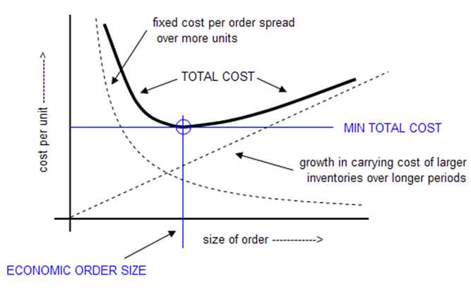
Production runs have fixed costs which are amortized over the number of units produced in a run. The cost per unit of fixed costs goes down as the number of units in a run goes up. Counteracting the economy of scale are the costs that result from longer runs. The most quantifiable costs resulting from long runs are inventory carrying costs. Longer runs will result in higher average inventories as long as the rate of consumption is less that the rate of production. So far, the question of the most economic run length is framed as a traditional supply chain economic order quantity (EOQ) problem. EOQ problems are solved by equations that capture the relationships shown in the graph below. A minimum overall cost is found at the low point of the total cost curve. EOQ analysis can be misleading since the consequences of forecast error and supply chain misallocation are not considered.

Supply chain impact

Cycle stock is that part of a production run that is not consumed downstream during the production run. The amount of cycle stock each run is the product of the length of the run and the difference between the production rate and the consumption rate.

Deployment of cycle stock

Companies with multiple supply chain echelons must decide where to deploy cycle stock. For example, if cycle stock of an intermediate product is produced at a plant there may be three options:

• Hold cycle stock in bulk at the plant and package as needed
• Package cycle stock into finished goods and store at plant
• Ship cycle stock downstream to company distribution centers

The choice among these options is often driven by the availability of storage space at the plant. If storage space is scarce, cycle stock will be shipped to company distribution centers (DC's).

Allocation of deployed cycle stock

In the above example, in order to package cycle stock, an allocation must be made among the finished items that can be produced from the bulk material. Depending on the production cycle, this allocation may require a forecast of demand weeks or months in advance. A consequence of less accurate allocation is that one of the finished items made from the bulk material will run out sooner. This, in turn will result in a shorter production cycle, and higher overall average inventory levels.

In order to ship cycle stock of finished goods downstream, it must be allocated to DC's. Misallocation to DC's may result in the need for redeployment as some DC's run out of the product while others have excess amounts.

Impact of forecast error

Greater forecast error increases the cost of downstream allocation of cycle stock. Unfortunately, the very products likely to have a high ratio of cycle stock to throughput are the ones with relatively low demand. These SKU's also tend to have highly variable and unpredictable demand.

Resource utilization

It is common for the systems where run length is of greatest concern to also be the capacity limiting echelon of the supply chain. Longer runs provide less scheduling flexibility and therefore lead to the need for additional safety stock to protect downstream inventories from the fact that the start of a production run may be delayed in order to complete a prior run.

Test Case

Company X has four plants producing 14 brands on five mixing systems. These systems feed packaging lines that produce 18 SKU's. Customers are supplied from seven company owned DC's; a few customers are supplied directly from the plants. Each DC is assigned to a primary plant. During times of demand over capacity, plants can shift demand to other plants that make the same product. When demand is over capacity system wide, product is pre-built to meet the anticipated excess demand.

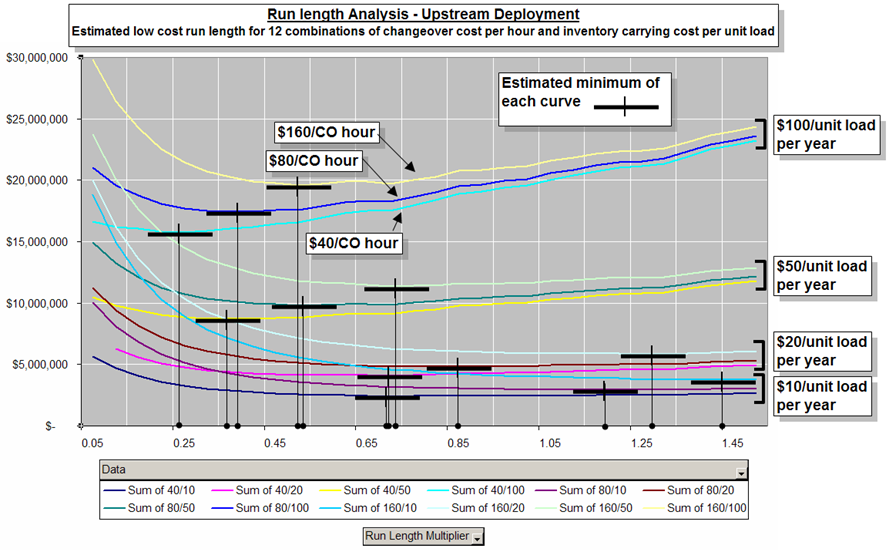
The impact of varying production run lengths was assed on changeover costs, inventory costs and customer service. The findings of this study can be found in Impact of Run Length on Supply Chain Performance. The following is a sample chart from the paper:

Production Capacity

Summary

In many industries, product demand varies substantially during the course of the year. It may not be cost effective to size productive capacity to match demand peaks. Aside from increasing capacity to cover periods of maximum demand, there are four potential responses to periods of demand over capacity:

• Shaping demand to flatten out peaks
• Extend production hours by using overtime during the week and on the weekends.
• Transfer production to other plants that have excess capacity

Other plants may not normally be preferred because production or shipping costs may be higher.

Capacity Management Strategies

1. Demand Shaping

   Demand shaping broadly entails efforts to match demand with productive capacity. Demand management techniques include customer incentives, reseller incentives, and sales compensation.

   For a concise summary of current practices, see Best Practices in Demand Shaping by Oracle.

   Simulation provides an effective tool for assessing combinations of production and demand scenarios.

2. Overtime

   The first recourse in dealing with periods of demand over capacity is to add production shifts, requiring overtime. Simulation allows assessment of the trade-off between increasing capacity and reducing the need for overtime.

   

Case Studies

• Life Cycle Resource Management Model The primary purpose of this model is to study the consequences of a mismatch between capacity and life cycle peak demand. The only strategy available to cope with periods of capacity under demand was pre-building.
• Inventory Deployment Model In this model the first line of defense against plant capacity falling short of demand was transferring demand to another less efficient plant. If capacity system wide was under demand, prebuilds were scheduled.
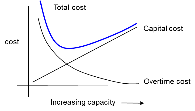
• Chemical Packaging Model A central issue in the chemical packaging model was the need for overtime. The tradeoff between capital cost of increases capacity and the cost of overtime was assessed.

Flexible ordering

Summary

Proven Methodology: SDI has conducted extensive independent research on flexible ordering benefits, detailed in our paper: Safety Stock Savings from Flexible Order Contracts: A Simulation Study

Our benchmark studies demonstrate that flexible ordering can achieve up to 77% of maximum potential safety stock savings through strategic contract design, with savings highly sensitive to flexibility in early contract periods.

Ordering arrangements for products with long lead times and demand variability can benefit both the buyer and the seller by including provisions for revision of order quantities after the order is initially placed.

'Flex Ordering' allows the buyer to place an order with substantial lead time, say 22 weeks, but then revise the quantity of the order within windows and percentages specified in the flex ordering contract. This benefits the buyer by reducing the safety stock that would be required to protect against higher than expected demand. It benefits the supplier by providing a degree of predictability of production requirements.

Assessment

Assessment of potential savings

In an independent study of flexible ordering conducted by Simulation dynamics, a test case was used with an overall lead time of 22 weeks. Safety stock savings at the customer end were assessed across combinations of the following factors:

• Customer order fill goal
• Customer forecast error variation
• Start week of flex periods (the order is fixed for some period before delivery)
• Flexibility allowed in each flex period
• Duration of flex periods

Maximum savings available

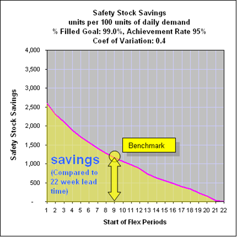
The chart below shows the maximum savings available under one set of assumptions. These are the savings if infinite flexibility were given until the onset of the fixed order period. For example, the benchmark shown at nine weeks indicates a maximum savings of 1200 units of safety stock. This case is the equivalent of having a nine week lead time. As the fixed order period is reduced to zero, the potential savings increases.

Potential Savings

The study looked at the percent of this maximum savings that would be achieved by various combinations of flex ordering contract parameters.

Findings

Sensitivity to flex percent	Sensitivity to length of flex periods	Mixed flex rates
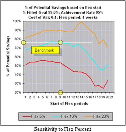
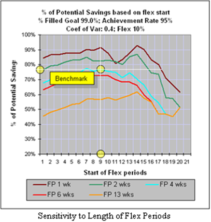
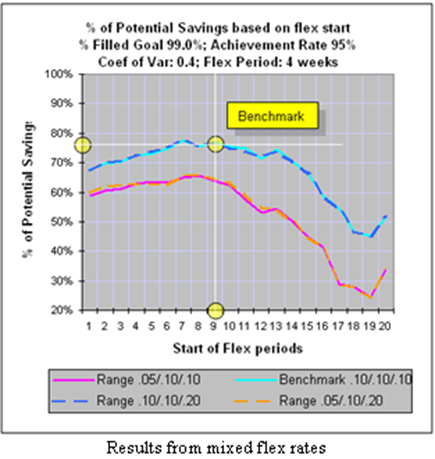
The plot below shows the percent of potential savings that result from our benchmark flex ordering design, starting in week 9, with four week periods of 10% flex. About 77% of the potential savings is realized. In addition, the percentage of potential savings is shown for the same flex design but with 5% and 20% flex.	The plot below compares our benchmark case to flex designs with different lengths of flex period. In each of these cases, the flex increase and decrease amounts are 10%. Case FP1 has flex periods of one week. This means that flex amounts could be increased or decreased each week. For example, with FP1, an order of 700 units could be increased thirteen times by week 9 to a quantity of 1610 units. FP13 is a design with only one flex period: each order can only be increased or decreased by a total of 10%.	The plot below shows the sensitivity of savings to changes in the flex rate of the first and third periods of the benchmark flex contract design. The results shown here indicate that safety stock savings are very sensitive to changes in flex rates in the first flex period, while not sensitive at all to changes in the third period.

Conclusions

The goal of this study was to gain insight into the sensitivity of the benefits of flexible ordering to several exogenous and endogenous factors. We have determined that the potential for savings is a function of:

• Order lead time
• Customer order filling goals
• Demand variability
• Start of flex periods

The amount of this potential that is realized is a function of:

• Length of flex periods (number of periods)
  • Shorter flex periods result in greater savings
• Percent of flex increase and decrease
  • Increase and decrease both contribute to savings
  • Flexibility in early periods is far more important than in later periods
  • Increase flexibility has greater benefits as demand variability increases

The goal of a negotiated flex ordering arrangement would be to find the lowest total cost to buyer and supplier, with a reasonable division of the savings over conventional fixed contracts. This study views flex ordering from the buyer's perspective. In such a negotiation, if the buyer has the ability to determine the savings from alternative proposed contracts, and has the supplier's proposed cost for such contracts, an informed decision can be made as to which contract has the best combination of cost and performance for the buyer. In addition to highlighting the factors that contribute to savings from flex ordering, this paper suggests that simulating inventory behavior under alternative flex ordering schemes would provide valuable support in such a negotiation.

Case Studies

• Life Cycle Resource Management Model Flexible ordering was used as a primary tool to reduce large safety stocks at the US assembly plant. The need for large safety stocks results from long lead times results from short term demand unpredictability.